radial.lib
Library of radials filters used with Ambisonics up to degree $L = 10$.
- Near-Field (NF) filters
- Near-Field Compensation (NFC) filters
- Rigid sphere diffraction filters
Theoretical background
Near-Field filters
The Ambisonics components for a point source (spherical wave) with signal $S$, at wavenumber $k = \frac{2 \pi f}{c}$ ($f$ being the frequency and $c$ the sound speed), and located at $(r_s, \theta_s, \phi_s)$ are given by:
\[\begin{equation} B_{l,m} = S F_{l}(k r_s) Y_{l,m}(\theta_s, \phi_s), \label{eq:blm} \end{equation}\]In Eq. \eqref{eq:blm} $F_{l}(k r_s)$ is the Near-Field (NF) filter1 at degree $l$, radius $r_s$, given by:
\[\begin{equation} F_{l}(k r_s) = \frac{e^{- i k r_s}}{r_s} \sum_{n=0}^{l} \frac{(-i)^n}{l! (kr_s)^n}\frac{(l+n)!}{(l-n)!}, \label{eq:nf} \end{equation}\]where $i = \sqrt{-1}$.
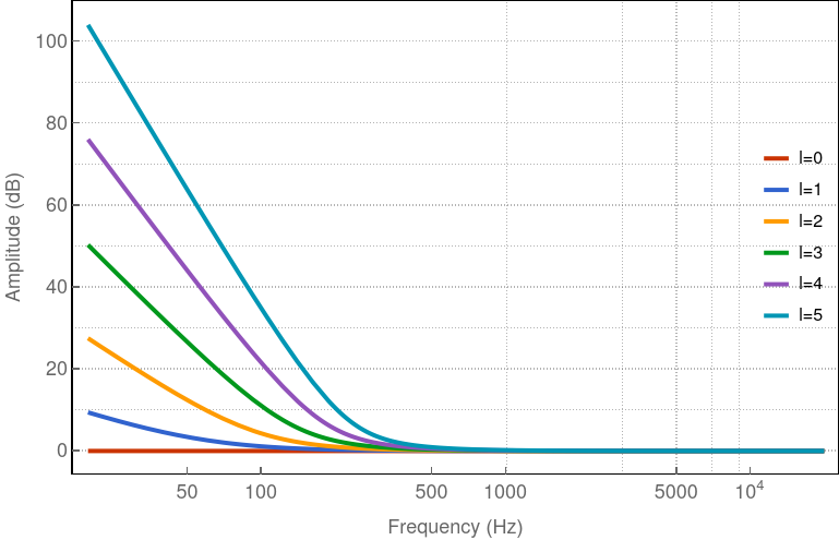
An illustration of $F_{l}$ is shown in Fig. 1 for $r = 1$ m and $l \in \{0, 1, 2, 3, 4, 5\}$. The filters $F_{l}$ are not feasible as such as they present a infinite gain at $k r_s = 0$.
Near-Field Compensation filters
Consider a loudspeaker array with $N$ loudspeaker, modeled as point source. For this array, the decoder matrix is denoted $\mathbf{D} \in \mathbb{R}^{(L+1)^2 \times N}$ and is working up to degree $L$. The driving signal of the $n$-th loudspeaker, located at a radial distance $r_\text{spk}$ is denoted $s_n$. It is given at wavenumber $k$ by:
\[\begin{equation} s_n = \sum_{l=0}^L \frac{1}{F_l(k r_\text{spk})} \sum_{m=-l}^l D_{n, l, m} B_{l, m} \label{eq:spk} \end{equation},\]where $\frac{1}{F_l(k r_\text{spk})}$ is the Near-Field Compensation (NFC) filter1 at degree $l$, and $D_{n, l, m}$ is the $(l, m)$ term of the $n$-th row of the matrix $\mathbf{D}$.
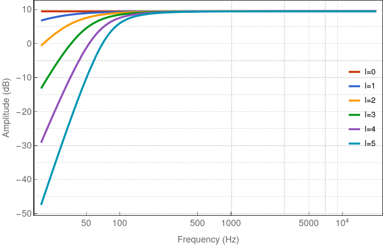
An illustration of $F_{l}$ is shown in Fig. 2 for $r_\text{spk} = 3$ m and $l \in \{0, 1, 2, 3, 4, 5\}$.
The NFC filters are accessible with the function nfc. Note that the negative delay $e^{i k r_\text{spk}}$ in Eq. \eqref{eq:nf} is not modeled in the current implementation.
Stabilization of NF filters with NFC filters
In practice, the NF filters at radius $r_s$ are stabilized with the NFC filters at radius $r_\text{spk}$.
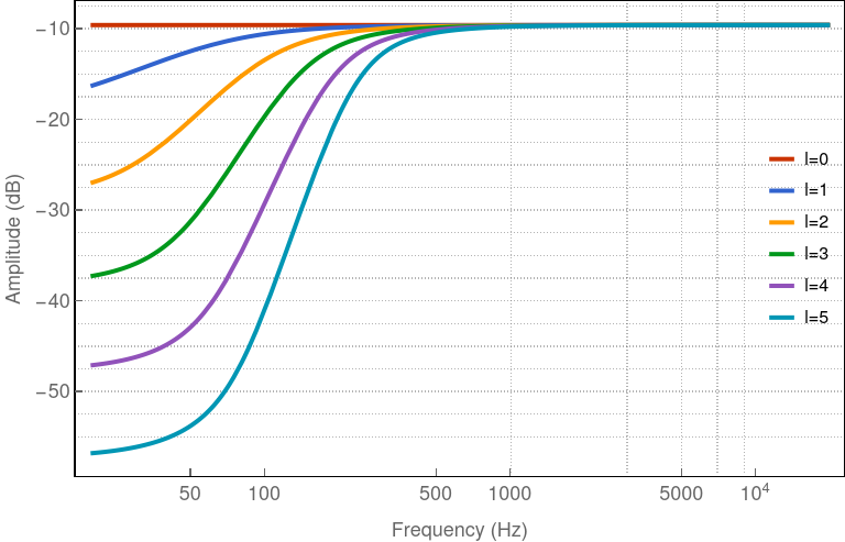
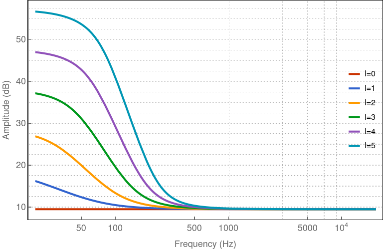
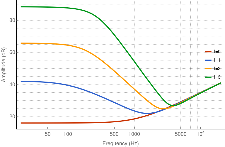
The resulting filters $\frac{F_l(k r_s)}{F_l(k r_\text{spk})}$ are shown for a $r_s > r_\text{spk}$ in Fig. 3 and $r_s < r_\text{spk}$ in Fig. 4.
In the latter case, note that the gain can be extremely loud at low frequencies and higher degrees $l$ and eventually damage the loudspeakers ! This is the so-called “Bass-Boost” effect1.
The filters $\frac{F_l(r_s)}{F_l(r_\text{spk})}$ are accessible with the function nf.
Rigid sphere diffraction filters
When retrieving the Ambisonic components with a rigid Spherical Microphone Array (SMA) of radius $r_\text{sma}$, the rigid sphere diffraction has to be compensated. This is done by applying the filter $E_l$ as follows:
\[\begin{equation} B_{l,m} = E_l(k r_\text{sma}) p_{l,m} \end{equation},\]where $p_{l,m}$ is the Spherical Fourier Transform (SFT) of the pressure measured on the SMA surface. The filters $E_l$ are given by:
\[\begin{equation} E_l(k r_\text{sma}) = i^{1 - l}(k r_\text{sma})^2 h'_l (k r_\text{sma}). \end{equation}\]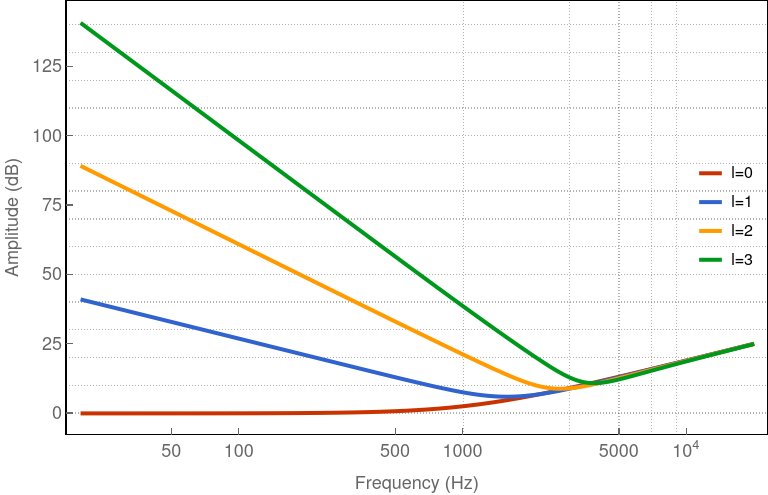
The filters $E_l(k r_\text{sma})$ are shown or $r_\text{sma} = 49$ mm and $l \in \{0, 1, 2, 3\}$ in Fig 5. They present an unreasonable amplification at low frequency and high degree $l$. They are not feasible as they present a infinite gain a $k r_\text{sma} = 0$.
Stabilization of rigid sphere diffraction filters with NFC filters
In practice, the filters $E_l$ at radius $r_\text{sma}$ are stabilized with the NFC filters at radius $r_\text{spk}$.
The resulting filters $\frac{E_l(k r_\text{sma})}{F_l(k r_\text{spk})}$ are shown for a $r_\text{sma} = 49$ mm and $r_\text{spk} = 0.5$ m in Fig. 6.
Note that the gain can be extremely loud at low frequencies and higher degrees $l$.
The filters $\frac{E_l(r_\text{sma})}{F_l(r_\text{spk})}$ are accessible with the function eq.
Functions
nf(l,r1,r2)
Computes the filters $\frac{F_l(r_s)}{F_l(r_\text{spk})}$
nfc(l,r)
Computes the NFC filters $\frac{1}{F_l(r_\text{spk})}$
eq(l,r1,r2)
Computes the filters $\frac{E_l(r_\text{sma})}{F_l(r_\text{spk})}$.
ddelay(r)
Applies a smooth delay corresponding to propagation time $\lceil r/c \rceil$.