grids.lib

A library that provides the directions $(\theta, \phi)$ and weights $w$ of several spherical grids, used in Spherical Microphone Arrays (SMA) configurations, or for regular decoders. Each grid works up to a specific degree $L$ of decomposition for a band limited function ($ \leq L$) on the sphere. If the function on the sphere is not band-limited, as the acoustic pressure, spatial aliasing occurs¹.

Functions

lebedev(N, i, x)

Gives the direction or weight of a $N$-node Lebedev grid. The Lebedev grids allows for an exact integration of spherical harmonics on the sphere up to a degree $L$². In the current implementation, 4 grids are provided as follows:

Number of Nodes $N$	Maximum working degree $L$
6	1
14	2
26	3
50	5

Note that the grid are nested¹: The first $6$ nodes of lebedev(50, i, x) corresponds to the $6$ nodes of lebedev(6, i, x), the first $14$ nodes of lebedev(50, i, x) corresponds to the $14$ nodes of lebedev(14, i, x), and so on.

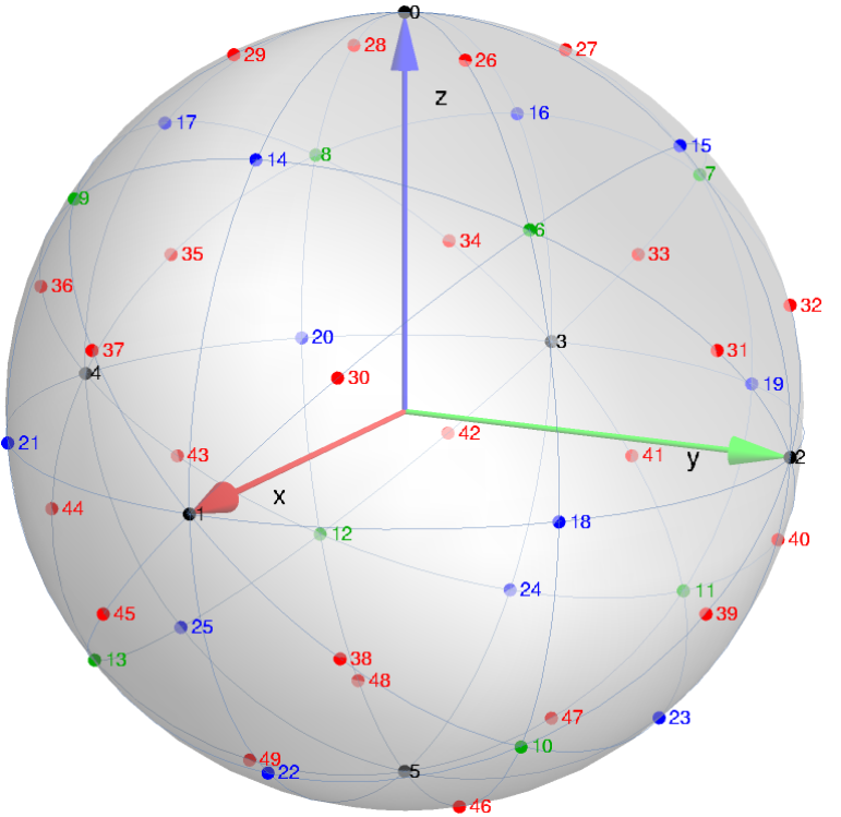
The nodes are indexed by the following order of priority: category, then polar angle $\phi$, then Azimuth angle $\theta$. Each node’s direction is given in the following table. An illustration is shown in Fig.1.

Node index $i$	Azimuth $\theta$ ($^\circ$)	Elevation $\phi$ ($^\circ$)
0	0	90
1	0	0
2	90	0
3	180	0
4	-90	0
5	0	-90
6	45	35
7	135	35
8	-135	35
9	-45	35
10	45	-35
11	135	-35
12	-135	-35
13	-45	-35
14	0	45
15	90	45
16	180	45
17	-90	45
18	45	0
19	135	0
20	-135	0
21	-45	0
22	0	-45
23	90	-45
24	180	-45
25	-90	-45
26	45	65
27	135	65
28	-135	65
29	-45	65
30	18	18
31	72	18
32	108	18
33	162	18
34	-162	18
35	-108	18
36	-72	18
37	-18	18
38	18	-18
39	72	-18
40	108	-18
41	162	-18
42	-162	-18
43	-108	-18
44	-72	-18
45	-18	-18
46	45	-65
47	135	-65
48	-135	-65
49	-45	-65

Usage: lebedev(N, i, x) where:

• N: number of node. $N \in \{ 6, 14, 26, 50\}$.
• i: node index, with $0 \leq i < N$.
• x: node direction or weight, as follows:
  • 0: node azimuth angle $\theta$,
  • 1: node elevation angle $\phi$,
  • 2: node weight.

---

em32(i,x)

Gives the direction or weight for a 32-node mh acoustics em32 Eigenmike® SMA. The grid corresponds to a Pentakis-Dodecahedron.

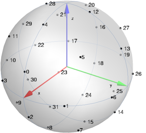
The node are sorted according to the em32 documentation³. Each node’s direction is given in the following table. An illustration is shown in Fig.2. The grid works up to degree $L=4$.

Node index $i$	Azimuth $\theta$ ($^\circ$)	Elevation $\phi$ ($^\circ$)
0	0	21
1	32	0
2	0	-21
3	-32	0
4	0	58
5	45	35
6	69	0
7	45	-35
8	0	-58
9	-45	-35
10	291	0
11	-45	35
12	91	69
13	90	32
14	90	-31
15	89	-69
16	180	21
17	-148	0
18	180	-21
19	148	0
20	180	58
21	-135	35
22	-111	0
23	-135	-35
24	180	-58
25	135	-35
26	111	0
27	135	35
28	-91	69
29	-90	32
30	-90	-32
31	-89	-69

Usage: em32(i,x) where:

• i: node index, with $0 \leq i \leq 31$.
• x: node direction or weight, as follows:
  • 0: node azimuth angle $\theta$,
  • 1: node elevation angle $\phi$,
  • 2: node weight.

---

zm1(i,x)

Gives the direction for a 19-node Zylia ZM-1 SMA. The grid corresponds to a Dodecahedron minus a node.

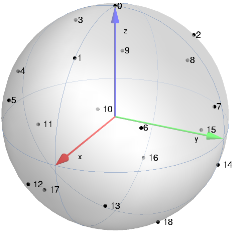
The node are sorted according to the Zylia ZM-1 documentation⁴. Each node’s direction is given in the following table. An illustration is shown in Fig.3.

Node index $i$	Azimuth $\theta$ ($^\circ$)	Elevation $\phi$ ($^\circ$)
0	0	90
1	0	48
2	120	48
3	-120	48
4	-82	19
5	-38	19
6	38	19
7	82	19
8	158	19
9	-158	19
10	-142	-19
11	-98	-19
12	-22	-19
13	22	-19
14	98	-19
15	142	-19
16	-180	-48
17	-60	-48
18	60	-48

zm1dsft(i)

Returns the $i$-th line of the Discrete Spherical Fourier Transform (DSFT) matrix (or encoding matrix) for the zm1 grid, i.e. the matrix that projects the acoustic pressures measured by the zm1 SMA on the spherical harmonics. This matrix, denoted $\mathbf{Y}_\text{DSHT} \in \mathbb{R}^{(L+1)^2 \times Q}$ is defined as the Moore-Penrose pseudo-inverse of the matrix $\mathbf{Y} \in \mathbb{R}^{Q \times (L+1)^2}$ of spherical harmonics evaluated up to the degree $L=3$ in the $Q=19$ directions of the zm1 grid nodes⁵:

\[\begin{equation} \mathbf{Y}_\text{DSFT} = \mathbf{Y}^\dagger = (\mathbf{Y}^T \mathbf{Y})^{-1} \mathbf{Y}^T, \end{equation}\]

where $^T$ is the transpose operator and

\[\begin{equation} \mathbf{Y} = \left[ \begin{array}{ccc} Y_{0,0}(\theta_0,\phi_0) & \cdots & Y_{L,L}(\theta_0, \phi_0) \\ \vdots & \vdots & \vdots \\ Y_{0,0}(\theta_{Q-1}, \phi_{Q-1}) & \cdots & Y_{L,L}(\theta_{Q-1}, \phi_{Q-1}) \end{array} \right]. \end{equation}\]

Usage: zm1dsft(i) where:

• i: row number with $[0 \leq i \leq 15]$.

cart2spher(x,y,z)

Computes the spherical coordinates $(r, \theta, \phi)$ from the Cartesian coordinates $(x, y, z)$ as:

\[\begin{equation} \begin{aligned} & r = \sqrt{x^2 + y^2 + z^2} \\ & \theta = \arctan\left( \frac{y}{x} \right) \\ & \phi = \arcsin\left( \frac{z}{r} \right) \end{aligned} \end{equation}\]

---